Getting Started with the International Disaster Database (EM-DAT) using Python and Pandas

Over the past few weeks I’ve been exploring the International Disaster Database (EM-DAT), which provides data on over 25,000 mass disasters from the year 1900 to present day.

I first came across the database after discovering Juliana Negrini de Araujo’s fantastic Jupyter Notebook which provides some high-level exploration of the dataset.

In many ways, the EM-DAT dataset is my first foray into analyzing natural disasters with Python.

I’ve spent some time building on Juliana’s work, cleaning up some code, and providing some additional detail and commentary — today I’m excited to publish the article. I hope it helps the community, and at the very least, it serves as documentation for myself as I continue exploring the EM-DAT dataset.

Overall, the goal of this article is to provide a detailed introduction to the EM-DAT natural disaster dataset, serving as a starting point for anyone else in the community who wants to study natural disasters through a data science lens.

Download the code

• All code published on NaturalDisasters.ai can be found in the official GitHub repo.
• The code for this specific article can be found here.

What is the EM-DAT database, and what is used for?

The EM-DAT dataset catalogs over 26,000 mass disasters worldwide from 1900 to present day.

EM-DAT is maintained by the Centre for Research on the Epidemiology of Disasters (CRED), and is provided in open access to any person or organization performing non-commercial research.

It is critical to understand that EM-DAT does not catalog all natural disasters worldwide. It instead focuses on mass disasters.

According to EM-DAT and CRED, a mass disaster is a specific type of natural disaster that leads to significant human and economic loss, requiring that at least one of the following criteria hold:

• 10 fatalities
• 100 affected people
• A deceleration of state of emergency (at the country level)
• A call for international assistance (again, at the country level)

For example, if a tornado touches down in rural Texas but doesn’t kill anyone, nor does it cause significant property damage, then the tornado would not be added to the EM-DAT dataset.

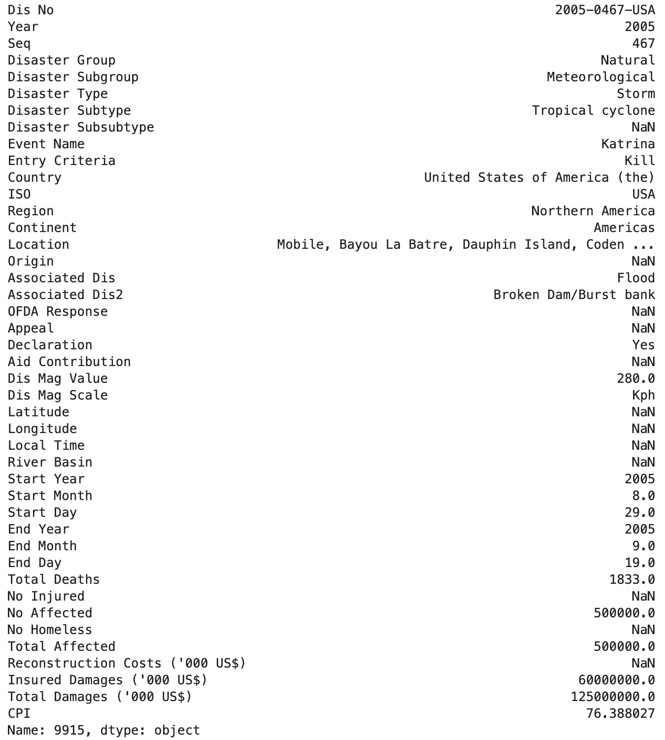
An example of a mass natural disaster that would be included in the the EM-DAT dataset is Hurricane Katrina, which absolutely devastated New Orleans, LA, and the surrounding areas, causing over 1,800 fatalities and estimated damages in the range of $98-145 billion USD.

Clearly, Hurricane Katrina passes multiple tests for inclusion in the EM-DAT dataset.

Below, I’ve included the data EM-DAT reports for Hurricane Katrina so you can get a feel for the data EM-DAT provides:

It’s also worth nothing that EM-DAT utilizes a hierarchical classification of all disasters, as I discuss in the “Breaking down disaster types in the EM-DAT dataset” section of the article.

One particular benefit of the hierarchical structure is that you can “drill down” into natural disaster type based on the following taxonomy:

1. Disaster Group
2. Disaster Subgroup
3. Disaster Type
4. Disaster Subtype
5. Disaster Subsubtype

Let’s take “extreme storms” as an example:

• The Disaster Group is Natural for all rows (at least for the Kaggle version of the dataset)
• The Disaster Subgroup for a storm is Meteorological
• The Disaster Type is then storm
• We then have multiple Disaster Subtypes that we can explore, including Convective Storm, Extra-tropical Storm, and Tropical Cyclone
• And finally, we can drill down further into the Disaster Subsubtype. A Convective Storm as the following subsubtypes: Derecho, Hail, Lightning/Thunderstorms, Rain, Sand/Dust storm, Severe storm, Storm/Surge, Tornado, and Winter storm/Blizzard

Using Python and Pandas, we can easily filter the natural disasters we are most interested in.

EM-DAT data at a glance

Exploring the EM-DAT dataset (image credit)

Approximately two-thirds of disasters recorded in EM-DAT are related to natural hazards.

Here are common occurrences for natural hazards in the dataset:

• Drought: 790
• Earthquake: 1,570
• Extreme temperature: 600
• Flood: 5,750
• Landslide: 790
• Storm: 4,580
• Volcanic activity: 270
• Wildfire: 450

As you can see, the EM-DAT dataset is quite diverse, covering a wide variety of natural disasters.

While there are certainly other datasets that provide far more data for a specific natural disaster type (for example, NOAA’s dataset on tornadoes), there are few datasets like EM-DAT that provides worldwide natural disaster data for such a diverse collection of disaster types.

The diversification factor alone makes EM-DAT worth studying in more detail (at least in my humble opinion).

Limitations of the EM-DAT dataset

The EM-DAT dataset is not without its limitations (image credit)

I want to be upfront and say that working with the EM-DAT dataset can be a bit challenging at times:

• The dataset is noisy.
• Many of the features have missing/incomplete data, with seven columns in particular having > 90% of the features missing.
• The data can also be inconsistent and non-standardized, particularly when it comes of the location of where a natural disaster occurred.

For example, when working with location data in the United States, some rows will have a mixture of:

• Region of the US (East, West, Southwest, etc.)
• State
• County
• City
• Town

Much of this location data is mixed and matched, making it sometimes challenging to work with.

Note: In fact, I had to develop a separate AI-based script to clean up the location data (which I’ll provide in a future article).

While EM-DAT strives to maintain high data accuracy, it relies on multiple sources for its data, including:

• United Nations agencies
• Non-government organizations
• Insurance companies
• Research institutions
• Press agencies
• etc.

Each of these organizations has its own reporting standards which may or may not facilitate high data accuracy.

Additionally, the estimates on economic loss data can vary significantly, implying that the economic loss estimates EM-DAT reports may not measure the full extent of the natural disaster impact.

Finally, and in my opinion, most importantly, under-reporting can be a concern when utilizing EM-DAT in your work or research.

By design, EM-DAT only includes natural disasters where:

1. 10 or more people are killed
2. 100 or more people were affected
3. A state of emergency was declared
4. A call of international assistance was issued

By definition, these exclusion criteria may result in natural disasters not being included in the dataset (but otherwise should be) due to limited media coverage, lack of money/infrastructure to gather reliable data, etc.

The EM-DAT is an invaluable resource, but it does have its limitations, so keep them in mind if you choose to utilize it in your own work;

Understanding each of the columns/features in the EM-DAT dataset

The EM-DAT dataset includes 43 features (i.e., columns) used to represent and quantify mass natural disasters worldwide.

I’m still exploring and wrapping my head around the nuanced contextualization of each of these features, but I’ve done my best to summarize each of them below:

1. Dis No: Unique identifier for each recorded disaster event.
2. Year: The year the disaster occurred.
3. Seq: Sequence number representing the occurrence order of events in a given year.
4. Disaster Group: Broad categorization of the disaster (e.g., natural or technological).
5. Disaster Subgroup: More specific category within the main disaster group (e.g., biological, climatological, hydrological, etc.).
6. Disaster Type: Specific type of disaster (e.g., wildfire, flood, storm, etc.)
7. Disaster Subtype: Further subclassification of disaster type (e.g., forest fire, flash flood, tropical cyclone, etc.).
8. Disaster Subsubtype:: Even more detailed classification within the subtype (e.g., mudslide, blizzard, tornado, etc.).
9. Event Name: Name given to the disaster event, if any (e.g., Tropical Storm Noul, Typhoon Molave, etc.).
10. Entry Criteria: Criteria that justified the event’s inclusion in the database.
11. Country: Country where the disaster occurred.
12. ISO: The ISO code representation of the country (e.g., USA, SRB, YEM, etc.).
13. Region: Geographical or administrative region within the country (e.g, Northern America, Southern Europe, Caribbean, etc.).
14. Continent: The continent where the disaster took place.
15. Location: Specific location or city affected by the disaster (note: this column is very inconsistent — values range from state/province, city, county, etc.).
16. Origin: Root cause or source of the disaster (e.g., heavy rains, earthquake, landslide, etc.).
17. Associated Dis: Related disaster events, if any (e.g., famine, industrial accident, heat wave, etc.).
18. Associated Dis2: Secondary related disaster events.
19. OFDA Response: U.S. Office of Foreign Disaster Assistance’s response, if any (values are either yes or NaN).
20. Appeal: Any international appeals for assistance (values are either yes, no, or NaN).
21. Declaration: Declarations made regarding the disaster (values are either yes, no, or NaN).
22. Aid Contribution: Amount of aid contributed (reported in thousands of US dollars) in response to the disaster.
23. Dis Mag Value: Numeric value representing the magnitude of the disaster (must be used in conjunction with Dis Mag Scale to properly interpret).
24. Dis Mag Scale: Scale used to measure the disaster’s magnitude, such as KPH, Richter, etc. For example, if Dis Mag Value has a value of 110, and Dis Mag Scale reports KPH, then the natural disaster was reported as having a (presumed) wind speed of 110 KPH.
25. Latitude: Geographic latitude of the disaster’s epicenter or main affected area.
26. Longitude: Geographic longitude of the disaster.
27. Local Time: Local time when the disaster occurred or was first reported.
28. River Basin: The river basin affected (only applicable for flood events).
29. Start Year: Year the disaster event started.
30. End Year: Month the disaster event started.
31. Start Day: Day the disaster event started.
32. End Year: Year the disaster event ended.
33. End Month: Month the disaster event ended.
34. End Day: Day the disaster event ended.
35. Total Deaths: Total number of deaths caused by the disaster.
36. No Injured: Number of individuals injured due to the disaster.
37. No Affected: Number of individuals affected in any way by the disaster.
38. No Homeless: Number of individuals rendered homeless by the disaster.
39. Total Affected: Combined total of injured, affected, and homeless individuals.
40. Reconstruction Costs (‘000 US$): Estimated costs in thousands of US dollars for reconstruction after the disaster.
41. Insured Damages (‘000 US$): Estimated damages in thousands of US dollars covered by insurance.
42. Total Damages (‘000 US$): Total estimated damages in thousands of US dollars due to the disaster.
43. CPI: Consumer Price Index at the time of the disaster, useful for adjusting costs over time.

Again, I want to reiterate that these explanations are provided at the best of my knowledge given my current understanding of the dataset.

If you are already an expert in the EM-DAT dataset (or better yet, a curator of the dataset), please leave a comment below to correct any of my unfortunate (but well intentioned) misgivings.

Performing an exploratory data analysis of EM-DAT

When confronted with a new dataset that I have no prior experience with, I first like to perform an Exploratory Data Analysis (EDA) to better understand and summarize its main characteristics.

“In statistics, exploratory data analysis is an approach of analyzing data sets to summarize their main characteristics, often using statistical graphics and other data visualization methods”

Wikipedia - Exploratory Data Analysis

To start, I like to build a basic table that provides a summary of the following information:

1. Samples: Number of rows in the dataset
2. Features: Number of columns (i.e., what exactly is quantified and represented in the dataset)
3. Duplicate Rows: Number of rows that have entirely identical feature/column values as other rows (typically we want to remove duplicated rows, but that is often dataset dependent)
4. Rows with NaN: Total number of rows that have missing/not a number (NaN) values
5. Total NaNs: Total number of NaNs in the dataset (i.e., sum of all NaNs across all rows and all columns)

The following code loads the EM-DAT dataset from disk:

# import the necessary packages
from collections import namedtuple
import matplotlib.pyplot as plt
import seaborn as sns
import pandas as pd
import os

# specify the path to the EM-DAT dataset
emdat_dataset_path = os.path.join(
    "natural-disasters-data",
    "em-dat",
    "EMDAT_1900-2021_NatDis.csv"
)

# load the EM-DAT natural disasters dataset from disk
df = pd.read_csv(emdat_dataset_path)
df.head()

Note: For the sake of simplicity (and to ensure you can reproduce my results), I am using the version of the EM-DAT dataset hosted on Kaggle rather than the one provided by Centre for Research on the Epidemiology of Disasters (which requires registration).

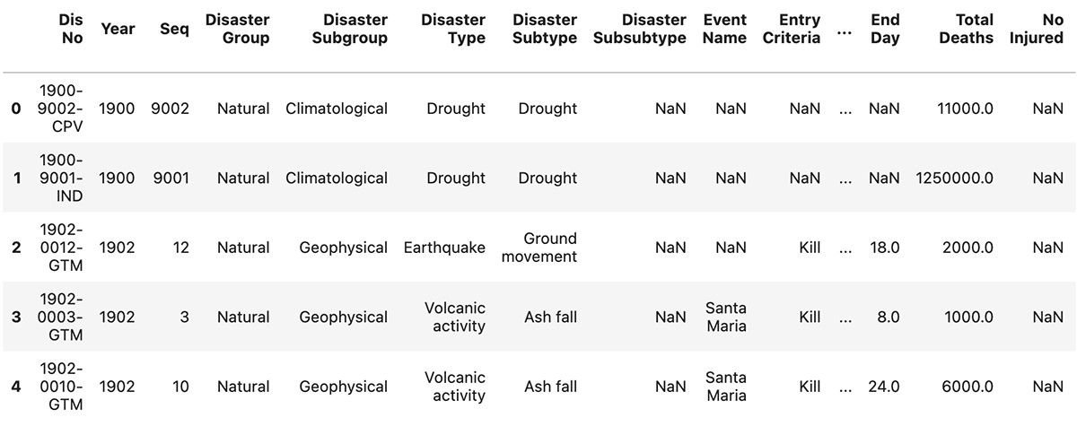
Below are the first five rows of the dataset:

A few noteworthy items:

• Notice how EM-DAT records mass natural disasters starting from the year 1990
• Disasters are categorized in a hierarchical fashion, starting from Disaster Group, and then working its way down to more fine-grained classifications via Disaster Subgroup, Disaster Type, Disaster Subtype, and Disaster Subsubtype
• Total deaths are reported
• The vast majority of feature values are missing/NaN

Below is my basic exploratory data analysis function (which I optimized from Juliana’s original implementation):

def basic_eda(df):
    # count the number of duplicated rows, then grab all NaN (i.e., null) rows
    # in the dataframe
    num_duplicated = df.duplicated().sum()
    is_nan = df.isnull()
    
    # count the total number of rows that contain *at least one* null value
    num_null_rows = is_nan.any(axis=1).sum()
    
    # count the total number of null values across *all* rows and *all* columns
    # (i.e., a sum of a sum)
    num_total_null = df.isnull().sum().sum()

    # construct a named tuple to represent each row in the exploratory data
    # analysis summary
    EDARow = namedtuple("EDARow", ["Name", "Value", "Notes"])

    # build the list of exploratory data analysis rows
    rows = [
        EDARow("Samples", df.shape[0], ""),
        EDARow("Features", df.shape[1], ""),
        EDARow("Duplicate Rows", num_duplicated, ""),
        EDARow("Rows with NaN", num_null_rows, "{:.2f}% all rows".format(
            (num_null_rows / df.shape[0]) * 100)),
        EDARow("Total NaNs", num_total_null, "{:.2f}% feature matrix".format(
            (num_total_null / (df.shape[0] * df.shape[1])) * 100)),
    ]
        
    # build and return our exploratory data analysis dataframe
    return pd.DataFrame(rows, columns=["Name", "Value", "Notes"])

The above code builds a summary dataframe.

An aspect of the code I want to point out is the difference between:

1. Counting the number of rows that have at least one null value (num_null_rows)
2. Counting the total number of NaN values across all rows and all columns (num_total_null)

The former is accomplished simply by summing the number of rows that have at least one null column.

I accomplish the later by doing two sums:

1. Count the number of NaN values in each row
2. Summing the sum of row-based NaN counts

The final dataframe provides the following information:

1. Number of rows (i.e., samples)
2. Number of columns (i.e., features)
3. Number of duplicate rows
4. Number of rows with NaN values
5. Total number of NaN values in the feature matrix

I can then call the basic_eda method on the EM-DAT dataset:

# perform a basic exploratory data analysis of the EM-DAT dataset
basic_eda(df)

Which provides the following summary table:

As the EDA table demonstrates, there are a total of 15,827 rows in the EM-DAT dataset.

Note: Again, I want to stress that I’m using the Kaggle version of the EM-DAT dataset, which is easily accessible and ensures you can reproduce any of my results. You can also use the CRED version of EM-DAT, which is also official version, but will require you to register before you can access it.

There are 43 features (i.e., columns) in the EM-DAT dataset (each of which I did my best to summarize earlier in this article).

The EM-DAT dataset has zero duplicate rows, meaning that no two rows in the dataset have identical column values.

Earlier in this article I mentioned that the EM-DAT natural disaster dataset is noisy, containing missing and incomplete data — the final two rows in the EDA table provide evidence to this claim.

First, every single row in the dataset has at least one column with a NaN value, meaning that there is no row with all column/feature values provided.

Additionally, approximately 42% of the entire feature matrix (15827 x 43 = 68,0561) is also NaN, implying that nearly half the dataset contains null values.

Datasets with a large number of NaNs can be quite challenging and problematic to work with for data scientists as we need to define how to handle missing values:

• Do we ignore rows with missing values? Keep in mind that every row of EM-DAT has a NaN value, so if we took this approach, we’d have an empty dataset.
• Do we try to impute (i.e., replace) missing values? That is certainly an option, but given that 42% of the feature matrix is incomplete, we’d be artificially filling in a large number of values, thereby calling into question the value and authenticity of the dataset.
• And if we decide to fill in missing values, what algorithms do we use? There are a plethora of data science algorithms that can be used to fill in missing values. How did we choose the right one?

In many cases, the answer is dataset (and even feature/column) dependent.

I’ve found that some of EM-DAT features can be reliably filled in while others cannot. I’ll likely do a future article on this type of study.

Investigating missing and unique values in EM-DAT

Given that 42% of all values in EM-DAT are missing, I found it worthwhile to spend a bit more time investigating exactly which features have values provided, and which ones are predominantly NaN.

Furthermore, I wanted to understand the uniqueness of the features, as unique values can have predictive power in downstream machine learning models.

To that end, I again built on Juliana’s work, and defined the summarize_data function to further summarize the EM-DAT dataset:

def summarize_data(df):
    # initialize a summary dataframe consiting of the original dataframe's
    # column names and data types
    summary = pd.DataFrame(df.dtypes, columns=["dtypes"])
    
    # reset the summary index, rename the "index" column to "Name", and then
    # remove the "index" column
    summary = summary.reset_index()
    summary["Name"] = summary["index"]
    summary = summary[["Name", "dtypes"]]
    
    # count the number of (1) null values for each column, and (2) the unique
    # values in each column
    summary["Missing"] = df.isnull().sum().values
    summary["Uniques"] = df.nunique().values
    
    # return the summary dataframe
    return summary

The summarize_data method constructs a dataframe that analyzes every column of the dataset.

For each column, four values are provided:

1. The name of the feature/column
2. The data type (integer, float, generic object, etc.)
3. Number of rows that contain a missing value for the particular feature
4. Number of unique values for the particular feature

Calling summarize_data on the df is as simple as:

# summarize the EM-DAT dataframe
summarize_data(df)

Which provides the following large block of output, analyzing the total number of missing and unique values for each column:

However, I find looking at such a table tedious and uninformative.

A more useful exercise is to visualize the above information.

Exploring features with missing values in EM-DAT

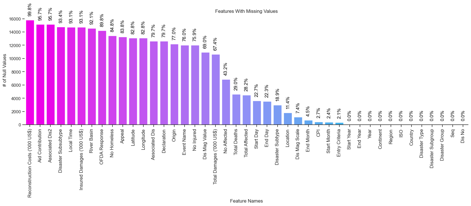
In my opinion, a better way to explore features with missing values is to count the number of NaN values per column, and then create a bar chart that plots the counts in descending order.

Doing so makes it trivially easy to identify columns with a large number of missing values with a simple visual inspection.

The following plot_null_columns method is more verbose, but provides a nicer, cleaner analysis:

def plot_null_columns(
    df,
    title,
    x_label="Feature Names",
    y_label="# of Null Values",
    figsize=(20, 5)
):
    # count the number of times a given column has a null value
    null_cols = df.isnull().sum().sort_values(ascending=False)
    
    # initialize the figure, set the tick information, and update the spines
    plt.figure(figsize=figsize)
    sns.set(style="ticks", font_scale=1)
    plt.xticks(rotation=90, fontsize=12)
    sns.despine(top=True, right=True, bottom=False, left=True)

    # plot the data
    ax = sns.barplot(x=null_cols.index, y=null_cols, palette="cool_r")

    # set the x-label, y-label, and title
    ax.set_xlabel(x_label)
    ax.set_ylabel(y_label)
    plt.title(title)

    # loop over the patches and null column counts
    for (p, count) in zip(ax.patches, null_cols):
        # compute the percentage of the number of rows that have a null value
        # for the current column
        ax.annotate(
            "{:.1f}%".format((count / df.shape[0]) * 100),
            (p.get_x() + (p.get_width() / 2.0), abs(p.get_height())),
            ha="center",
            va="bottom",
            rotation="vertical",
            color="black",
            xytext=(0, 10),
            textcoords="offset points"
        )

What I found tricky about the above code block is figuring out the computation of null_cols such that it could also be provided to the barplot method to plot the number of columns with missing values in descending order.

The trick was to first compute a column-wise count of NaNs, sort them in descending order (via sort_values), and then provide null_cols.index to the barplot function.

Secondly, I find it extremely helpful to also plot the percentage of null counts for each column directly above each of the individual bars — the for loop handles that computation.

The handy plot_null_columns function can then be called via:

# plot the null column counts within the dataset
plot_null_columns(df, "Features With Missing Values")

Which produces the following plot:

Clearly, it’s far easier to visually identify features with missing values using this approach.

A quick inspection of the above plot reveals there are seven features where over 90% of values are missing for a particular column, including:

1. Reconstruction Costs
2. Aid Contribution
3. Associated Dis2
4. Disaster Subsubtype (which makes sense given that we are performing a hierarchical categorization of natural disaster types, and many don’t need such a fine-grained categorization)
5. Local Time
6. Insured Damage
7. River Basin

Conversely, there are twelve features that I would consider form the “core definition” of the EM-DAT dataset:

1. Start Year
2. End Year
3. Year
4. Continent
5. Region
6. ISO
7. Country
8. Disaster Type
9. Disaster Subgroup
10. Disaster Group
11. Seq
12. Dis No

All twelve of these features contain values (i.e., non are missing/NaN), and while these values may still be noisy, they are at least present in the EM-DAT dataset.

In my initial studies I’ve predominately focused on these core features.

Understanding EM-DAT’s natural disaster hierarchy grouping

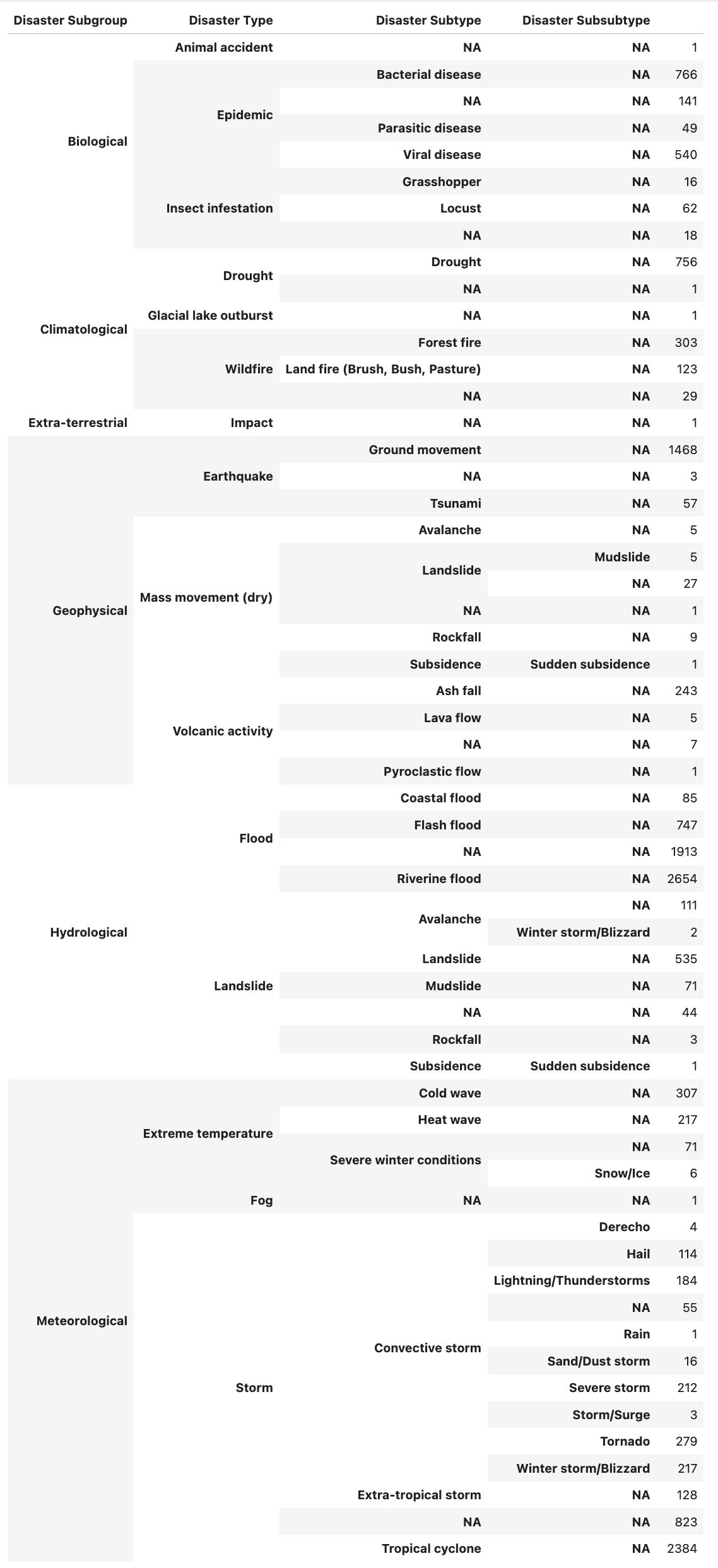
My initial foray into the EM-DAT dataset concluded with an exploration of the natural disaster hierarchy grouping using Disaster Group as the base, and then becoming more fine-grained based on:

1. Disaster Subgroup
2. Disaster Type
3. Disaster Subtype
4. Disaster Subsubtype

I found the hierarchy exploration absolutely essential in understanding EM-DAT’s structure, and if you’re exploring EM-DAT for the first time, I’d suggest you spend considerable time here.

Below is the code I used:

# define the disaster type columns we are interested then
disaster_cols = [
    "Disaster Subgroup",
    "Disaster Type",
    "Disaster Subtype",
    "Disaster Subsubtype",
]

# grab the disaster data from the dataframe
disaster_df = df[disaster_cols]

# fill any null values with an empty string (implying that no subgroups or
# subtypes exist for the current value)
disaster_df = disaster_df.fillna(value={
    "Disaster Subtype": "NA",
    "Disaster Subsubtype": "NA",
})

# construct the final dataframe which displays a hierarchical overview of the
# disaster types, including the counts for each one
disaster_df = pd.DataFrame(
    disaster_df.groupby(disaster_cols).size().to_frame("count")
)
disaster_df

Basically, what I’m doing here is:

1. Selecting only the hierarchical disaster_cols from the dataframe
2. Filling in any NaN values with a string (we don’t want to use a blank/empty string here because we want to be able to easily spot empty values in the hierarchy grouping in our output table)
3. Building an output table that summarizes the hierarchy

The groupby function call is doing quite a bit, but the gist is that the code groups the dataframe by the unique combinations of disaster_cols, counting the occurrences of each combination. The final counts for each combination are stored in a new column named count.

Running the above code produces the following table which concisely depicts the hierarchical organization of natural disasters in EM-DAT:

For example, let’s investigate the “Biological” subgroup — there are three disaster types for this subgroup:

1. Animal accident
2. Epidemic
3. Insect infestation

Now, let’s further examine the “Insect infestation” disaster type:

1. There are 16 occurrences of grasshopper infestations
2. 62 occurrences of locust infestations
3. And finally, there are 18 occurrences of when no further subtype is provided (and are assumed to be more “generic”, or at the very least, uncategorized, types of insect infestations).

I had to sit and study this hierarchy table for a bit to fully appreciate and understand the EM-DAT disaster categorization hierarchy.

If you’re considering working with EM-DAT, I’d highly suggest you spend at least 30-60 minutes here before you move on to more detailed data analysis.

If I hadn’t taken the time to understand the data hierarchy, I think I would have struggled considerably when I moved on to more advanced analysis.

Takeaways

• The International Disaster Database (EM-DAT) offers data scientists a rich dataset for the analysis of mass natural disasters, cataloging over 26,000 global events from 1900 to the present day.
• EM-DAT focuses specifically on mass disasters, defined as events leading to significant human and economic loss. Lesser incidents are not accounted for in the database.
• EM-DAT utilizes a hierarchical classification for disasters, allowing a detailed analysis based on categories such as Disaster Subgroup, Disaster Type, Disaster Subtype, and Disaster Subsubtype.
• While the database is a valuable resource, it does have limitations. A significant portion of the data includes missing or incomplete information, and specific categories like the precise location of a disaster can prove inconsistent and challenging to work with.
• Nevertheless, if you’re interested in studying natural disasters, I’d suggest starting with EM-DAT as the dataset is easy to use once you wrap your head around the basic structure (which this article attempted to do).

Citation information

Adrian Rosebrock. “Getting Started with the International Disaster Database (EM-DAT) with Python and Pandas”, NaturalDisasters.ai, 2023, https://naturaldisasters.ai/posts/getting-started-em-dat-international-disaster-database/.

@incollection{ARosebrock_GettingStartedEMDAT,
    author = {Adrian Rosebrock},
    title = {Getting Started with the International Disaster Database (EM-DAT) using Python and Pandas},
    booktitle = {NaturalDisasters.ai},
    year = {2023},
    url = {https://naturaldisasters.ai/posts/getting-started-em-dat-international-disaster-database/},
}

AI generated content disclaimer: I’ve used a sprinkling of AI magic in this blog post, namely in the following sections:

1. Understanding each of the columns/features in the EM-DAT dataset: I needed to summarize what each of the columns/features in the dataset represents. In order to create this summary, I fed my notes from each column into ChatGPT and had it summarize my findings into a nicely formatted numbered list.
2. Takeaways: AI was used to create a bulleted summary of the article.

Don’t fret, my human eyeballs have read and edited every word of the AI generated content, so rest assured, what you’re reading is as accurate as I possibly can make it. If there are any discrepancies or inaccuracies in the post, it’s my fault, not that of our machine assistants.

Header photo by NASA on Unsplash